Mathematical Definition of Image Classification Problem
Image classification is a task aimed at categorizing images into their respective labels.
This objective is typically addressed using neural networks. In this blog post, we have a dual purpose. Firstly, we will delve into the mathematical modeling of this problem from an optimization perspective. Secondly, we will demonstrate how to implement a custom one-hidden-layer linear neural network using PyTorch. We’ll also provide visualizations of the classification results and showcase the evolution of weights before and after training.
1. Image Classification Problem
Original Problem
In -class image classification problem (ICP), we are given a training dataset comprising pairs of images and labels, denoted as , where . Here, each image is represented as a 2D array of numbers with a size of , and label is the class of image . Notice that by flattening , one can consider as a usual column vector in . The main objective is to determine a label function that associates each image with its corresponding label , i.e.
In the following sections, we will explore how to model the function and how to deal with e the notion of approximation in equation (ICP1).
Reformulation
In the real world, we may not always know how to definitively classify an image into a specific class. Instead, we might express that belongs to each class with different probabilities. We will now demonstrate how to reformulate (ICP1) using this probabilistic approach.
Let represent the unit basis vectors in . Define as the simplex in . In this context, represents the space of probability distributions over the labels , where .
For a given image , let denote the probabilities associated with each label, where the entry stands for the probability that image belongs to label . By doing this, if if and only if is the label of with a probability of .
Consequently, we may encode label by vector :
Thus, in the following, we will consider the dataset instead of .
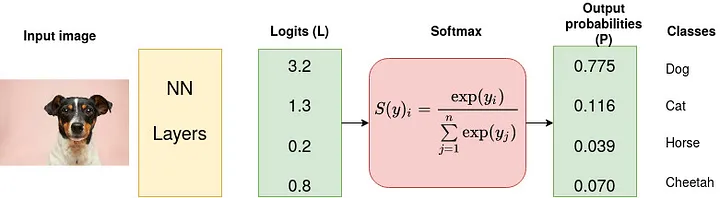
On the other hand, we notice that any function can be normalized to obtain a probability function as follows:
where the softmax function is defined by:
Naturally, we can define a label function as the index with the highest probability in , i.e.:
The problem (ICP1) can then be reformulated as follows: Given the dataset , for , our objective is to:
Optimization Approach
As finding a function across the space of general functions appears to be infeasible, we constrain to a set of parametric functions, denoted as , where represents a set of parameters. Achieving a function that satisfies the approximation in (ICP2) involves minimizing a loss function. Essentially, the objective here is to discover a Neural Network (NN), which is a specific parametric function denoted as , such that minimizes the following optimization problem:
Recall that , for . A commonly used loss function in this classification approach is the Cross Entropy Loss, defined as:
Note that (ICP3) is a highly non-convex optimization problem and solving it using iterative methods such as gradient descent is known as the process of training a NN.
2. One-hidden-layer Linear Neural Network
In this example, we will illustrate how to solve this problem using PyTorch by implementing the simplest form of a neural network: a one-hidden-layer linear neural network (without activation functions).
The function is defined as:
Here, , , , and .
We will use MNIST (Modified National Institute of Standards and Technology Database), a widely-used collection of handwritten digit data. MNIST comprises 60,000 training images and 10,000 testing images, each being a grayscale image with dimensions of 28x28 pixels. The main classification task involves assigning each image to one of classes, representing the 10 digits with labels .
In this case, we have , , and can be arbitrarily chosen, referred to as the size of the hidden layer.
The custom implementation of NN is provided below. The full code can be found in my Github.
class LinearLayer(nn.Module):
    def __init__(self, input_size, output_size):
        super(LinearLayer, self).__init__()
        torch.manual_seed(102)
		rand_weights = 2*(torch.rand(output_size, input_size)-0.5)
		self.weights = nn.Parameter(rand_weights)

    def forward(self, x):
        # x.shape = (m, d)
        # W.shape = (n, d)
        W = self.weights
        result = x @ W.T
        return result

# Fully connected neural network with one hidden layer
class NeuralNet(nn.Module):
    def __init__(self, input_size, hidden_size, num_classes):
        super(NeuralNet, self).__init__()
        self.input_size = input_size
        self.l1 = LinearLayer(input_size, hidden_size)
        self.l2 = LinearLayer(hidden_size, num_classes)

    def forward(self, x):
        out = self.l1(x)
        out = self.l2(out)
        # no activation and no softmax at the end
        return out
Some optimal weights before training

Some optimal weights after training

Some predictions after training


