Solving Elastic-Net problem using Proximal Gradient Descent

The Python code of this post is available on my Github.

Problem definition

In this note, we consider the so-called Elastic-Net problem

$$\min_{x\in \mathbb R^n} \quad \frac{1}{2}||b-Ax||_2^2 + \lambda_1||x||_1 + \frac{\lambda_2}{2}||x||_2^2$$

where $b\in \mathbb R^m$ and $A \in \mathbb R^{m\times n}$, $\lambda_1, \lambda_2\geq 0$. The optimal solution to this problem is sparse if $\lambda_2$ is small. In particular, the Lasso problem corresponds to $\lambda_2=0$.

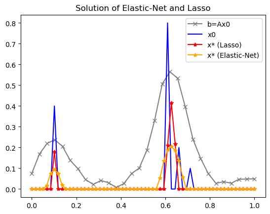
The following figures demonstrate the difference between the solutions of the Lasso and Elastic-Net problems. As you can see, the solution obtained through Lasso is sparser, while the solution obtained through Elastic-Net is smoother.

The evolution of iterative solutions of the two problems is

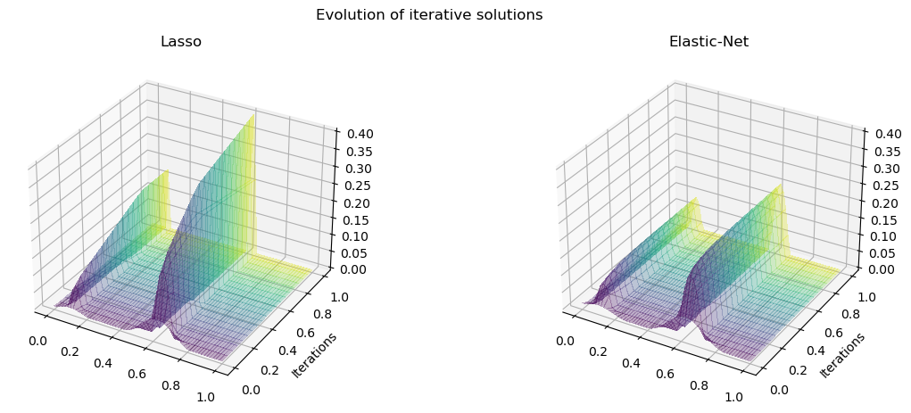
Solving method using Proximal Gradient Descent

The proximal gradient method is the following updating rule

$$x^{(k+1)} = \text{prox}_{g/\alpha} \left(x^{(k)} - \frac{1}{\alpha} \nabla f(x^{(k)})\right)$$

Here $\alpha>0$ is the Lipschitz constant of the gradient of $f$ (assuming that it exists), in this case $f$ is said to be $\alpha$-smooth.

Here let’s explain how such above update is a convergence algorithm.
Note that the Elastic-Net problem is a special case of the more general form

$$\min_{x} \quad P(x) = f(x) + g(x)$$

where $f$ is the main smooth loss function and $g$ is a regularization function which is usually non-smooth. If one assumes that $f$ has $\alpha$-Lipschitz continuous gradient then

$$P(x') \leq f(x) + \langle \nabla f(x), x'-x\rangle +\frac{\alpha}{2} ||x'-x||^2_2 + g(x') = M(x')$$

The function $M$ is called the surrogate function of $P$ with equality if $x'=x$. To minimize $P$ we can minimize $M$, this is known as the Majorize-Minimization method. To do that, let us rewrite $M$,

$$M(x') = f(x) - \frac{1}{2\alpha} ||\nabla f(x)||^2_2 + \frac{\alpha}{2} ||x' - x + \frac{1}{\alpha}\nabla f(x)||_2^2 + g(x')$$

Then, to minimize $M$ we apply the proximal operator on $g/\alpha$ with argument $x^+$, where $x^+ = x - \frac{1}{\alpha} \nabla f(x)$ is the gradient descent update from $x$, i.e.

$$\arg\min_{x'} \quad \frac{1}{2} ||x' - x^+||_2^2 + \frac{1}{\alpha} g(x') = \text{prox}_{g/\alpha} (x^+).$$

This is exactly the proximal gradient descent method described above.

Back to Elastic-Net problem

To apply the proximal gradient descent, we need the closed form expressions for $\alpha$, $\nabla f$ and $\text{prox}_{g/\alpha}$. This is a simple task.

For the Elastic-Net problem, we can choose $\alpha = ||A||^2_{Fro} = \sum_{i+1}^n ||a_i||_2^2$ the squared Frobenius norm, i.e. the total squared norms of the $i$-th column $a_i$ of $A$.

With $f(x) = \frac{1}{2} ||b - Ax||_2^2$, we have $\nabla f(x) = -A^T(b-Ax)$.

For $g(x) = \lambda_1||x||_1 +\frac{\lambda_2}{2}||x||_2^2$, we find the proximal associated with $g/\alpha$ as follows.

$$\arg\min_{x'} \quad \frac{1}{2} ||x' - x^+||_2^2 + \frac{\lambda_1}{\alpha}||x'||_1 + \frac{\lambda_2}{2\alpha} ||x'||_2^2$$

Let $s = \text{sign}(x')$, then the Fermat’s rule reads as follows

$$x' - x^+ + \frac{\lambda_1}{\alpha} s + \frac{\lambda_2}{\alpha} x'=0 \leftrightarrow x' = \frac{\alpha}{\alpha + \lambda_2} \left[x^+ - \frac{\lambda_1}{\alpha}s\right]$$

By considering different cases of sign of $x'$ and $x^+ \pm \frac{\lambda_1}{\alpha}$, we can eliminate $s$ in the formula of $x'$ as follows

$$\text{prox}_{g/\alpha}(x^+) = x' = \frac{\alpha}{\alpha + \lambda_2} \text{sign}(x^+) \left[|x^+| - \frac{\lambda_1}{\alpha}\right]_+.$$
This is the closed form expression for proximal of $g/\alpha$.