Knapsack Problem

1. Problem definition

Knapsack problem is defined as
$$\begin{aligned} \max \quad & \langle c, x\rangle\\ \text{s.t.} \quad & \langle 1, x\rangle =b\\ \quad & x\in [0, \overline x] \end{aligned}$$
Without loss of generality, we assume that $c$ is sorted, i.e. $c_1\geq c_2 \geq ....\geq c_n>0$. The solution of this problem has a closed form solution.
Let $k$ be the largest index so that
$$\gamma_k := \sum_{i=1, k} \overline x_i \leq b$$
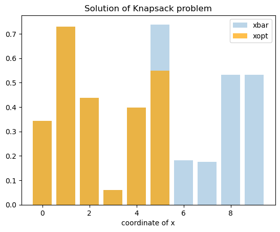
Then the optimal solution $x^\star$ can be characterized by $k$,
$$\begin{aligned} x^\star_i = \begin{cases} \overline x_i & \text{ if } i\leq k\\ b - \gamma_k & \text{ if } i= k+1\\ 0 & \text{ otherwise} \end{cases} \end{aligned}$$

The following figure demonstrates a solution of Knapsack problem.

2. Property of Knapsack

Let $\overline b = \sum_{i=1,n} \overline x$. It is clear that the Knapsack problem is feasible iff $b\in [0, \overline b]$. Let $f(b)$ be the maximum value of above Knapsack problem parameterized by $b$. Then we have the following theorem characterizes the function $f$

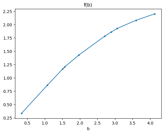
Theorem. The optimal value of knapsack problem $f$ is a piecewise linear increasing concave function of budget parameter $b \in [0, \overline b]$.

Moreover, the breakpoints of $f$ are $\gamma_k$ defined as above. On $[\gamma_{k-1}, \gamma_{k}]$, the slope of $f$ is $c_k$, which forms a decreasing sequence, thus $f$ is concave. The following figure demonstrates the graph of $f$.

3. Code

# 1. solving knapsack
import numpy as np 
np.random.seed(123)

n = 10
c = - np.sort(-np.random.rand(n)) # cost coefficients with decreasing order
xbar = np.random.rand(n) # bounds of x
lbd = 0.61 # parameter of b
b = lbd * xbar.sum() # budget

def knapsack(c, xbar, b):
	# c is sorted in decreasing order 
	# b <= sum(xbar)
	xopt = np.zeros_like(xbar) 
	gamma = 0 
	for i in range(n):
		gamma += xbar[i] 
		xopt[i] = xbar[i]
		if gamma >b:
			gamma -= xbar[i] 
			xopt[i] = b - gamma
			break
	return xopt
    
xopt = knapsack(c, xbar, b)
print("opt solution is", xopt)
print("check sum(xopt) = b, result is", np.abs(xopt.sum() - b)<1e-6)


# 2. vis knapsack solution
import matplotlib.pyplot as plt 
plt.bar(range(n), xbar, alpha=0.3, label="xbar")
plt.bar(range(n), xopt, alpha=0.7, color="orange", label="xopt")
plt.legend()
plt.xlabel("coordinate of x")
plt.title("Solution of Knapsack problem")
plt.show()

# 3. plot knapsack function 
gamma_values = []
S = 0
for i in range(n):
    S += xbar[i]
    gamma_values += [S] 

def max_knapsack(c, xbar, b):
    xopt = knapsack(c, xbar, b)
    max_value = np.dot(c, xopt) 
    return max_value 

f_values = [max_knapsack(c, xbar, b) for b in gamma_values]

plt.plot(gamma_values, f_values, marker=".")
plt.title("f(b)")
plt.xlabel("b")
plt.show()

Linear Programming using Interior Point Method

Linear programming is a method to optimize a linear objective function subject to linear constraints. The interior point method is an algorithm that can be used to solve linear programming problems by moving a point inside the feasible set.

Problem Statement

Consider the following linear programming problem:

$$\min_{x \in \mathbb{R}^n} c^T x$$

subject to

$$Ax≤b$$

where $c \in \mathbb{R}^n$, $A \in \mathbb{R}^{m \times n}$, and $b \in \mathbb{R}^m$.

Barrier Function

To use the interior point method, we need to define a barrier function that penalizes violation of the constraints. The convex barrier function $-\log$ is frequently used:

$$\phi(x) = - \sum_{i=1}^m \log (b_i - a_i^T x)$$

where $a_i^T$ is the $i$-th row of $A$.

The barrier function approaches infinity as $x$ approaches the boundary of the feasible region. Therefore, minimizing the barrier function ensures that $x$ stays inside the feasible region.

Interior Point Method

The interior point method solves the following optimization problem:

$$\min_{x \in \mathbb{R}^n} c^T x + \frac{1}{t}\phi(x)$$

where $t$ is a positive scalar called the barrier parameter.

The interior point method find $x$ for $t$ belongs to an increasing sequence, until convergence. At each iteration, it solves the above optimization problem (with a specific $t$) using Newton’s method.

Python Implementation

Here’s the Python code for solving the above linear programming problem using the interior point method. The produced figure is.

import numpy as np
import matplotlib.pyplot as plt
from scipy.optimize import minimize
import pypoman
from scipy.spatial import ConvexHull

# Define the objective function
c = np.array([-1, 0])  # coefficient of decision variables in the objective function

# Define the inequality constraints
A = np.array([[1, 2], [1, -1], [-1, 1], [-1, -1]])
b = np.array([2, 2, 2, 1])

# Define the function to be minimized
def objective(x):
    return np.dot(c, x)  # minimize c'x

# Define the barrier function and its Jacobian
def barrier(x):
    return -np.sum(np.log(b - np.dot(A, x)))

def jacobian_barrier(x):
    return np.dot(A.T, (1/ (b-A.dot(x))))

# Define the function to be minimized for the interior point method
def func_to_minimize(x, t):
    return objective(x) + barrier(x)/t

def jacobian_func(x, t):
    return c + jacobian_barrier(x)/t

# data container for x and t
x0 = np.array([0, 0])
x = x0
t = 1
x_list = [x]
t_list = [t]

# Implement the interior point method
for i in range(10):
    # Define the function to be minimized and its Jacobian
    func = lambda x: func_to_minimize(x, t)
    jac = lambda x: jacobian_func(x, t)
    
    # Solve the optimization problem
    res = minimize(func, x, method='Newton-CG', jac=jac)
    print(f"Iter={i}, success={res.success}, gap={2/t}")
    
    # Update t and x0
    t *= 1.8
    x = res.x.copy()
    t_list += [t]
    x_list += [x]

We then plot the figure

# Plot the movement of the solution point
fig, ax = plt.subplots()
vertices = pypoman.compute_polytope_vertices(A, b)
vertices = np.vstack(vertices) # shape (n, 2)
indices = ConvexHull(vertices).vertices
vertices = vertices[indices, :]

delta = 0.025
x_grid = np.arange(-2.0, 2.5, delta)
y_grid = np.arange(-2.0, 1.5, delta)
X, Y = np.meshgrid(x_grid, y_grid)
Z = np.zeros_like(X)


x_list = np.array(x_list)
levels = np.sort([func_to_minimize(x, t) for x, t in zip(x_list, t_list)])

def plot_contour(point, t):	
	for i in range(len(x_grid)):
		for j in range(len(y_grid)):
			Z[j, i] = func_to_minimize([x_grid[i], y_grid[j]], t)
	lev = [func_to_minimize(point, t)]
	ax.contour(X, Y, Z, levels=lev, colors='black', linewidths=1)
        
for point, t in zip(x_list, t_list):
    plot_contour(point, t)

ax.fill(vertices[:, 0], vertices[:, 1], color="cyan",
         alpha=0.3, edgecolor='black', linewidth=1)
ax.set_xlim([-2, 2.5])
ax.set_ylim([-2, 1.5])
ax.plot(x_list[:, 0], x_list[:, 1], 'o--', markersize=5)
ax.set_xlabel('x1')
ax.set_ylabel('x2')
ax.set_title('Interior Point Method for Linear Programming')
plt.show()