Gradient flow for Blasso problem

Note: This blogpost is the next part of the previous post about numerical methods for Blasso problem: Solving Blasso problem using gradient descent method.

Let $M(T)$ be the space of Radon measures supported on a compact set $T\subset \mathbb R^d$.

Blasso problem is
$$\min_{\mu \in M(T)}\quad \frac{1}{2}||b-A\mu||^2_H + \lambda ||\mu||_{TV},$$
where $b\in H$, $H$ is a Hilbert space, operator $A: M(T) \rightarrow H$ is linear and weak* continuous, $\lambda>0$ and $||\cdot||_{TV}$ the total variation norm of Radon measures.

Blasso is a non-smooth, convex optimization problem. It is an infinite-dimensional counterpart of the Lasso problem.

Under certain conditions (see Theorem 2 in Duval and Peyre), there exists an optimal measure being discrete, i.e., combination of a small number $n$ of Dirac masses:
$$\mu^* = \sum_{i=1}^n w_i \delta_{t_i}$$
for $w_i\in \mathbb R$ and $t_i\in T$.

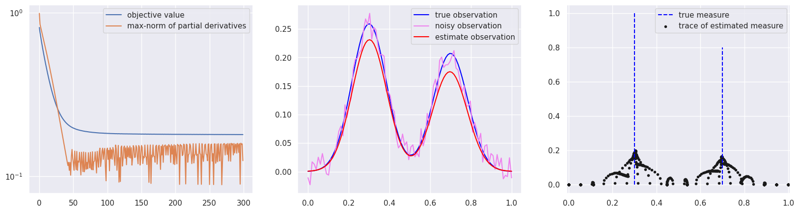
To solve this problem, the gradient flow method was proposed. Its basic idea is to approximate the unknown measure $\mu$ by a discrete measure with sufficiently large number $m$ ($m \gg n$) of Dirac masses and perform the simple gradient update (roughly speaking gradient flow) on the weights $w_i$ and $t_i$ for $i=1,..., m$.

This blog post modifies our previous python code and obtains the following numerical result, which confirms the convergence of discrete measures (black dots in the third figure).

The python code is provided below

import torch
import matplotlib.pyplot as plt
import seaborn as sns
sns.set_theme()

def dic(x, t, w):
    diff = x.reshape(-1, 1) - t.reshape(1, -1)
    g = torch.pow(2, -diff**2/w**2)
    norm = g.norm(p=2, dim=0)
    return g/norm


def opt_min(func, point, lr=1e-2, max_iters=500, epsilon=1e-2):
    point.clone()
    data = {
        "val": [],
        "grad_max": [],
        "points": []
    }

    for i in range(max_iters):
        point.requires_grad = True
        point.grad =  torch.zeros(point.shape)
        loss = func(point)
        loss.backward()
        grad = point.grad
        point = point - lr * grad
        # detach
        loss = loss.detach()
        grad = grad.detach()
        point = point.detach()
        # save
        grad_max = grad.abs().max()
        data["val"] += [loss]
        data["grad_max"] += [grad_max]
        data["points"] += [point.clone()]

        # stop
        if grad_max<epsilon:
            break

    return point, data


def test():
    x = torch.linspace(0., 1., 100)
    w =0.1

    p0 = torch.tensor([0.3, 0.7])
    c0 = torch.tensor([1., 0.8])
    y0 = dic(x, p0, w) @ c0.reshape(-1, 1)

    noise = 0.5*(torch.rand(y0.shape)-0.5)
    y = y0 + 1e-1 * noise

    lbd = 0.1

    t = torch.linspace(0., 1., 10)
    def func(point):
        p, c = point
        a = 0.5 * (y - dic(x, p, w) @ c.reshape(-1, 1)).norm()**2
        b = lbd * c.norm(p=1)
        return a+b

    p = torch.linspace(0., 1., 20)
    c=torch.zeros(len(p))
    point = torch.cat([p, c]).reshape(2, -1)
    point_est, data = opt_min(func, point,max_iters=300)


    p_est, c_est = point_est

    y_hat = dic(x, p_est, w) @ c_est.reshape(-1, 1)

    f, (ax1, ax2, ax3) = plt.subplots(1, 3, figsize=(20, 5))
    ax1.plot(data["val"], label="objective value")
    ax1.plot(data["grad_max"], label="max-norm of partial derivatives")
    ax1.set_yscale("log")
    ax1.legend()

    ax2.plot(x, y0.reshape(-1), label="true observation", color="blue")
    ax2.plot(x, y.reshape(-1), label="noisy observation", color="violet")
    ax2.plot(x, y_hat.reshape(-1), label="estimate observation", color="red")
    ax2.legend()

    ax3.vlines(x=p0, ymin=0., ymax=c0, label="true measure", color="blue", ls="--")
    # ax3.vlines(x=p_est, ymin=0., ymax=c_est, label="estimate measure", color="red", ls="--")
    for i in range(len(data["points"])):
        if i % 7 ==0:
            p = data["points"][i]
            if i==0:
                ax3.scatter(p[0], p[1], marker=".", c="k", label="trace of estimated measure")
            else:
                ax3.scatter(p[0], p[1], marker=".", c="k")

    ax3.set_xlim(-0.01, 1.01)
    ax3.legend()

    plt.show()


test()