Support Vector Machine (P1)

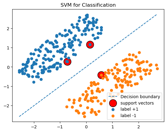
In this tutorial, we learn how to model the problem of classifying two clouds of data points as an optimization problem, which is known as the Support Vector Machines (SVM) problem. We also provide the Python code using Scikit-Learn to solve this problem.

SVM is a supervised machine learning algorithm used for classification tasks. It aims to find a hyperplane that separates the input data points based on their labels.

In the SVM problem, we are given a set of data points represented as $(x_i, y_i) \in \mathbb{R}^n \times \{-1, 1\}$, where $x_i$ is the input feature vector and $y_i$ is its corresponding label. The objective of SVM is to find a hyperplane associated with two parameters $(w, b) \in \mathbb{R}^n \times \mathbb{R}$ that can effectively separate the data points based on their labels. The hyperplane is defined as $P = \{x \in \mathbb{R}^n: \langle w, x\rangle + b = 0\}$, where $\langle w, z\rangle$ denotes the dot product of vectors $w$ and $z$.

The goal is to find the hyperplane $P$ that maximizes the margin between the data points of different classes. That is to maximize $\gamma$ defined as $$\gamma = \min_{i=1,..., n} \gamma_i,$$where $\gamma_i$ is the distance from $x_i$ to $P$.

To derive the formula for $\gamma_i$, we can assume without loss of generality that for $y_i=+1$, we have $\langle w, x_i\rangle + b\geq 0$, then let $z_i = x_i - \gamma_i \frac{w}{||w||}$ be the projection of $x_i$ onto $P$, then $z_i\in P$, that is $\langle w, z_i\rangle + b= 0$. Solving this equation we obtain $\gamma_i = (\langle w, x_i\rangle + b)/||w||$. Similar for $y_i=-1$. We then obtain
$$\gamma_i = \frac{y_i(\langle w, x_i\rangle + b)}{||w||}.$$

Therefore, to find $(w, b)$ we solve the following problem
$$\begin{aligned} \max_\gamma \quad & \gamma\\ \text{ s.t. } \quad & \frac{y_i(\langle w, x_i\rangle + b)}{||w||} \geq \gamma \end{aligned}$$

By the change of variable $w' = w/(\gamma ||w||)$ and $b' = b/(\gamma ||w||)$, we observe that $\gamma =1/||w'||$ and the problem is therefore equivalent to
$$\begin{aligned} \min_{w, b} \quad & \frac{1}{2}||w'||^2\\ \text{ s.t. } \quad & y_i(\langle w', x_i\rangle + b') \geq 1. \end{aligned}$$

Code

import numpy as np
from sklearn import svm
import matplotlib.pyplot as plt

# 1. Generate data
def rotate(p, origin=(0, 0), degrees=0):
    p = p.T
    angle = np.deg2rad(degrees)
    R = np.array([[np.cos(angle), -np.sin(angle)],
                  [np.sin(angle),  np.cos(angle)]])
    o = np.atleast_2d(origin)
    p = np.atleast_2d(p)
    return np.squeeze((R @ (p.T-o.T) + o.T).T).T

def generate_points():
	np.random.seed(12) 
	p = np.random.uniform(low=-2, high=2, size=(500, 2)).T

	margin = 0.7
	pos = p[1]>=margin
	neg = p[1]<=-margin
	x_pos = p[:, pos]
	x_neg = p[:, neg]
	x_pos = rotate(x_pos, origin=(0, 0), degrees = 45)
	x_neg = rotate(x_neg, origin=(0, 0), degrees = 45)
        
	return x_pos, x_neg

x_pos, x_neg = generate_points()
n = x_pos.shape[1] + x_neg.shape[1]
X = np.hstack([x_pos, x_neg]).T
y = np.hstack([- np.ones(x_pos.shape[1]), np.ones(x_neg.shape[1])])
print(X.shape, y.shape)


# Step 2: Create and Train the SVM Model
model = svm.SVC(kernel='linear')
model.fit(X, y)
support_vectors = model.support_vectors_.T
w = model.coef_[0][0]
b = model.intercept_[0]


# Step 3. Plot
x_min, x_max = X.T[0].min(), X.T[0].max()
x_grid =  np.linspace(x_min, x_max, 100)
y_values = w*x_grid + b 
plt.plot(x_grid, y_values, ls="--", label="Decision boundary")

plt.scatter(support_vectors[0], support_vectors[1], label = "support vectors", color="red", edgecolors='black', s=300)
plt.scatter(x_pos[0], x_pos[1], label = "label +1")
plt.scatter(x_neg[0], x_neg[1], label = "label -1")
plt.legend()
plt.title('SVM for Classification')
plt.show()