A deep understanding of PCA: From statistics to optimization explanation

Abstract. Principal Component Analysis (PCA) stands as a widely utilized technique for condensing high-dimensional data into a low-dimensional space while retaining the “maximum amount of information”. This post delves into the mathematical modeling of PCA through the lens of optimization rather than the other popular explanations based on statistics.

1. Introduction

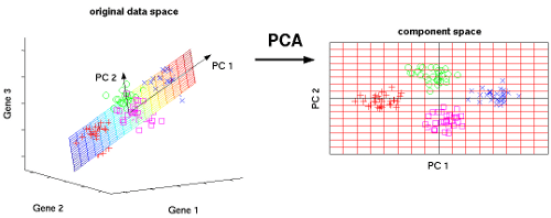
Principal Component Analysis (PCA) stands out as a widely embraced technique for transforming very high-dimensional datasets into a very low dimension while retaining the “maximum amount of information”, see the figures above, depicting the transformation from 2D to 1D [1] and 3D to 2D [2].

The post is structured as follows:

• The next section provides a brief explanation of PCA from a statistical perspective.
• Following that, we delve into the optimization approach to explain PCA, emphasizing its central theme in this post.
• The post concludes by offering insights through comments that draw connections between the two approaches.

2. Statistics approach

In statistical terms, PCA method involves transforming the original variables into a new set of uncorrelated variables known as principal components. In order to maximize the information in the low-dimensional space, these components represent linear combinations of the original variables and are arranged in a specific order: the first principal component (to the eigenvector associated with the largest eigenvalue of the covariance matrix) explains the maximum variance in the data, the second component (the eigenvector associated with the second largest eigenvalue) explains the maximum remaining variance orthogonal to the first, and so forth.

While this statistical explanation for PCA is simple, it masks the intricate relationships among the concepts of eigenvectors, eigenvalues, the covariance matrix, and the covariance matrix’s role in maximum information preservation.

To unravel these complexities, in the following section, we will employ an optimization approach to describe how the PCA method works and thus provide a profound understanding of PCA.

3. Optimization approach

Given $n$ data points $x_i$ in a high dimensional space $\mathbb R^d$ (large $d$). The goal of PCA is to represent these points using other $n$ points $z_i$ in a very low dimensional space $\mathbb R^k$ ($k\ll d$) spanned by $\{a_1,...., a_k\}\subset \mathbb R^d$, i.e.
$$x_i \approx \mu + Az_i, \, \forall i=1,..., n,$$
where $\mu\in \mathbb R^d$ and $A= [a_1,..., a_k] \in \mathbb R^{d\times k}$. Here we assume that $\{a_1,..., a_n\}$ forms an orthogonal setting, i.e. $$A^TA = I_k.$$

Here, the approximation $\approx$ needs to be defined in a manner that ensures the preservation of the “maximum amount of information.” Intuitively, this preservation can be achieved through a “regression” model, wherein we seek the hyperplane $\mu+Az$ that best fits the data points $x_i$. In this context, $z_i$ represents the projection of $x_i$ onto the hyperplane (refer to the figures above).

Let’s delve into the mathematical details. PCA is essentially equivalent to solving the following optimization regression problem [3]:

$$\min_{\mu, A, z_i}\quad \sum_{i=1}^n ||x_i-\mu - Az_i||_2^2 \tag{1}$$

The hard part of this problem is finding $A$ since it is relatively easy to find $\mu$ and $z_i$ according to the following formulas (see more details in [3]):
$$\mu = \frac{1}{n} \sum_{i=1}^nx_i$$
and $$z_i= A^T(x_i-\mu), \forall i=1,..., n.$$

Note that w.l.o.g. we may assume that $\mu=0$ (otherwise, we let $x_i:=x_i-\mu$). By the formula of $z_i$, the problem (1) now can be rewritten as follows:
$$\min_{A}\quad \sum_{i=1}^n ||x_i- AA^Tx_i||_2^2 \tag{2}$$

Expanding (2), the focus now is to maximize

$$\sum_{i=1}^n x_i^TAA^Tx_i = \sum_{i=1}^n ||A^Tx_i||_2^2 = \sum_{i=1}^ntrace(A^Tx_ix_i^TA) = trace(A^TSA)$$
where $||v||_2^2 = trace(vv^T)$ and $S = \sum_{i=1}^n x_ix_i^T$ is a (scaled) covariance matrix.

The problem of finding $A$ is now equivalent to
$$\max_{A}\quad trace(A^TSA) \quad \text{ s.t. } \quad A^TA=I_k.\tag{3}$$

Let us now focus a particular case of (3) when $k=1$ i.e. $A \equiv a\in \mathbb R^d$:
$$\max_{a}\quad a^TSa \quad \text{ s.t. } \quad ||a||_2=1.$$

The minimum value of this problem is the so-called “norm of operator” of $S$, which is exactly the maximum eigenvalue of $S$, see e.g. [4], while the minimizer is the corresponding eigenvector.

In general, let $S = U\Lambda U^T$, where $U=[u_1,.., u_d]$ a unit orthogonal matrix of eigenvectors, i.e. $U^TU=I_d$, and $\Lambda=diag(\lambda_1,..., \lambda_d)$ be the diagonal matrix of eigenvalues of $S$ such that $$\lambda_1\geq ... \geq \lambda_d\geq 0,$$ then optimal solution $A$ of (3) is

$$A = [u_1,..., u_k]^T diag(\lambda_1,..., \lambda_k) [u_1,..., u_k].$$

4. Conclusion

Through the lens of the optimization approach, it becomes evident that PCA can be conceptualized as a regression model. In this model, the high-dimensional data points $x_i \in \mathbb{R}^d$, are aptly represented by a lower-dimensional points $z_i \in \mathbb{R}^k$, through a linear relation $x_i \approx \mu + Az_i$, where $k \ll n$.

In other words, the aim of preserving the “maximum amount of information” of data points can be achieved by solving a regression model.

In this model, the optimal matrix $A$ is found to be constructed using the $k$ largest eigenvalues and their corresponding eigenvectors from the (scaled) covariance matrix of $x_i$. This connection unveils itself as a generalization of the well-known fact: the “norm of a (positive definite) matrix is the largest eigenvalue of that matrix.”

5. References

[1] step-step-explanation-principal-component-analysis
[2] explanation-of-principal-component-analysis
[3] PCA and LASSO
[4] operator-norm-is-equal-to-max-eigenvalue