Projection onto L1 ball

Projection onto L1 Unit Ball

In this post, we will learn how to use soft thresholding operator to derive the solution of closest point projection onto a unit ball defined by $\ell_1$-norm.

Problem Definition

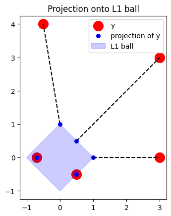
We are given a vector $y$ and want to find its projection onto the unit ball defined by the L1 norm. The problem can be formulated as an optimization problem:

$$\begin{aligned} \min \quad & \frac{1}{2} ||y - x||_2^2\\ \text{s.t.} \quad & ||x||_1 \leq 1 \end{aligned}$$

The following figure demonstrates the solution of above prolem.

Solving idea

Above problem can be solved with exact solution using soft threshold operator. To do this, we first notice that Lagrangian function is defined as

$$L(x, λ) = 1/2 ||y - x||_2^2 + λ(||x||_1 - 1)$$

It is known that if $x^\star$ is the optimal solution, then there exists $\lambda^\star$ so that $(x^\star, \lambda^\star)$ is a stationary point of the Lagrangian function. Assuming that $\lambda^\star$ is given, then $x^\star$ is a minimizer of $L(\cdot, \lambda^\star$, thus, it can be found using soft threshold operator $ST$,
$$x^\star = \text{ST}(y, \lambda^\star) = \text{sign}(y) [|y|-\lambda^\star]_+.$$

So the main problem now is finding $\lambda^\star$. To this end, we can use complementary slackness condition, which reads as follows $\lambda^\star (||x^\star||_1-1)=0$. Here, one can notice that if $\lambda^\star=0$ (this happens when $y$ belongs to the L1 ball), then $x^\star= y$. So we may assume that $\lambda^\star>0$, in this case, one can find $\lambda^\star$ by solving the following equation
$$||x^\star||_1- 1 = \sum_{i} [|y_i|-\lambda]_+-1=0.$$

In other words, we find $\lambda^\star$ by solving the equation $h(\lambda)=0$ for $\lambda \in [0, \lambda_{\max}]$, where $h(\lambda) = \sum_{i} [|y_i|-\lambda]_+-1$ and $\lambda_{\max}$ is some big number, that can be chosen by $\lambda_{\max}= ||y||_{\infty}$. The function $h$ is a piecewise convex function, that can be solved easily.

Experiment

# ref: https://math.stackexchange.com/questions/2327504/orthogonal-projection-onto-the-l-1-unit-ball

import numpy as np
import matplotlib.pyplot as plt 
def complementary_slackness(lbd, y):
    return np.sum(np.clip(np.abs(y) - lbd, a_min=0, a_max=None)) - 1

def get_breakpoints(y):
    lbd_min = 0
    lbd_max= np.max(np.abs(y))
    return np.sort(np.append(np.sort(np.abs(y)),[lbd_min, lbd_max]))

def find_lambda(y):
    # Find breakpoints of lambda and h(lambda) at these breakpoints 
    breakpoints = get_breakpoints(y)
    values = np.array([complementary_slackness(lbd, y) for lbd in breakpoints])
    if values[0]<=0:
        lbd_opt = 0
        return lbd_opt

    # Find adjacent breakpoints a, b so that f(a)>=0, f(b)<0 
    pos = values >= 0-1e-6
    indices = np.arange(len(values))
    a_index = indices[pos][-1]
    b_index = a_index +1 
    a = breakpoints[a_index]
    b = breakpoints[b_index]
    fa = values[a_index]
    fb = values[b_index]

    # Find optimal lbd by solving h(lambda) = 0
    # It is clear that lambda in [a, b]
    # This solution can be found using gamma-parameter equation
    # gamma*(a, fa) + (1-gamma)*(b, fb) = (solution, 0)
    gamma = -fb/(fa-fb)
    lbd_opt  = gamma*a+ (1-gamma)*b
    return lbd_opt
  
def plot_function_h(y, lbd_opt=None):
    # Find breakpoints of lambda and h(lambda) at these breakpoints 
    breakpoints = get_breakpoints(y)
    values = np.array([complementary_slackness(lbd, y) for lbd in breakpoints])

    # plot
    plt.plot(breakpoints, values, color="blue", marker=".", label="h(lambda)")
    plt.plot(breakpoints, np.zeros_like(breakpoints), color="gray")
    if lbd_opt is not None:
        plt.scatter(lbd_opt, 0, label="lambda_opt", color="red", s=100)
    plt.xlabel("lambda")
    plt.ylabel("h(lambda)")
    plt.legend()
    plt.show()

def soft_threshold(x, threshold):
    return np.sign(x) * np.maximum(np.abs(x) - threshold, 0)

def find_projection(y, lbd_opt):
    x_opt = soft_threshold(y, lbd_opt)
    return x_opt

We now simulate the graph of function $h(\lambda)$ and solve a 4 dimensional problem,

y = np.array([1,5,3,2])
lbd_opt = find_lambda(y)
plot_function_h(y, lbd_opt)
print(f"The projection point is x_opt = {find_projection(y, lbd_opt)}")
# x_opt = [0. 1. 0. 0.]

In the following, we provide the code to generate the figure at the beginning of the post.

# simulate data
y_points = [[3,3], [3, 0], [-0.5,4], [0.5, -0.5], [-0.7, 0]]
lbd_points = [find_lambda(y) for y in y_points]
x_points = [find_projection(y, lbd) for y, lbd in zip(y_points, lbd_points)]
segments = [([x[0], y[0]], [x[1], y[1]]) for x, y in zip(x_points, y_points)]

L1ball = [(1, 0), (0, 1), (-1, 0), (0, -1), (1, 0)]
L1ball0, L1ball1 = np.array(L1ball).T
y0, y1 = np.array(y_points).T
x0, x1 = np.array(x_points).T

# plot
plt.scatter(y0, y1, color='red', s=200, label="y")
plt.scatter(x0, x1, color='blue', s=30, label="projection of y")
plt.fill(L1ball0, L1ball1, color="blue", alpha=0.2, label="L1 ball")
for seg in segments:
    plt.plot(*seg, color="k", ls="--")
plt.title("Projection onto L1 ball")
plt.legend()
plt.axis('scaled')
plt.show()